I’d like to introduce a joint work with Junzhe Zhang and Elias Bareinboim, titled Sequential Causal Imitation Learning with Unobserved Confounders, which we presented at NeurIPS 2021. While the paper is a collaboration, the opinions and description here are my own.

This post is divided into 5 sections. The first is geared towards a general audience, and explains the problem’s basics. The second section shows how we encode this problem and how an answer would look, with the goal of being comprehensible to someone familiar with causal diagrams. The third section introduces imitation in sequential contexts, and the fourth section gives a taste of our contribution, geared towards a more technical audience. Finally, the post concludes with a brief discussion of our method’s limitations.

What Problem are we Solving?

Let’s use the example of building a self-driving car. Some carmakers are trying to develop these vehicles by gathering data on how humans drive, and then training a computer to behave the same way. In other words, with enough examples of people stopping at red lights, it is hoped that the machines will begin associating red lights with stopping, and behave correctly.

This is called imitation learning, because the machine (imitator) is being trained to copy a human (demonstrator). This problem has a strong theoretical foundation when both the demonstrator and the imitator see the same context (i.e. identical sensors), because with infinite data and exploration, the imitator will observe the environment and the demonstrator’s actions in every possible situation, and can then repeat the expert’s actions when acting itself!

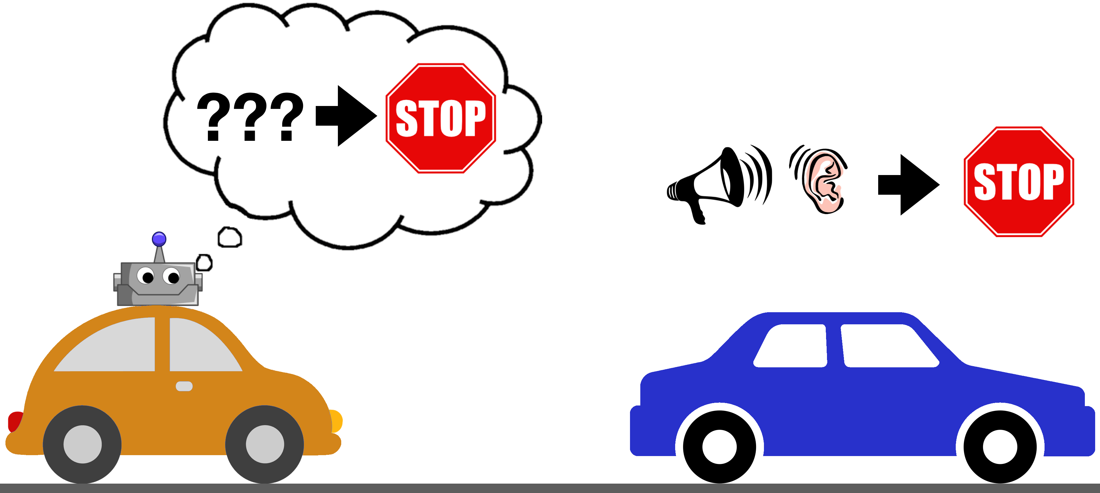
Things fall apart once the demonstrator and imitator have different views of the world, whether through different vantage points (a person sitting in back of a car doesn’t have a full view of the road) or different sensors (a deaf person won’t react to sounds). For example, current self-driving systems are based on cameras/lidar, and generally don’t include microphones. This means that while most human drivers (demonstrators) can hear and react to sounds, the self-driving car (imitator) cannot. What would happen if this deaf machine were trained to copy the behavior of a human driver who stopped their car after hearing screeching tires and people yelling? Since it might not see anything around it, it could conclude that a good driver should sometimes slam on the brakes for no reason!

Is there a way to avoid this type of situation? Can we have guarantees that the imitator will learn the right thing despite a mismatch in sensors and observations?

You might notice that when reasoning about the problem above, I told a story of how things were related, and what caused what. The person can hear, and sounds can reflect road conditions, which in turn can influence how the driver should behave. In order to approach the problem mathematically, we will encode this understanding of the world’s structure in a way that can be processed algorithmically.

When given a detailed description on how things are causally related, our method can then determine whether it is possible for the imitator to compensate for missing sensors. If such compensation is possible, the imitator can still have overall performance identical to that of the demonstrator, despite having a different view of the environment.

Causal Imitation

In our work, description of the environment is achieved using causal diagrams [1]. These acyclic graphs encode how variables in the system are related^[1]. To demonstrate, consider a continuation of the self-driving car example, where we are given a toy causal structure.

In this toy example, the car’s surroundings are represented by events to the front, back, and side of the car, and are drawn in the diagram below using F,B and S nodes. Whether or not someone is a good driver (reward, $Y$), is determined by the car’s surroundings (FBS), as well as the driver’s actions ($X$) in response to the surroundings. The events in the surroundings can cause there to be certain sounds, like screeching tires or car horns (H). Since the self-driving car (imitator) can’t hear, the H node is drawn with a dashed border. The human demonstrator, $X$ (blue) is looking forward (F), and can hear sounds (H) when performing their action.

In the ideal case, after observing the human’s driving for a while, we would then give the imitator ($X$ in orange) control over the car, with the same sensors. Unfortunately, since the imitator doesn’t have a microphone, it can’t hear car horns, and therefore has no way to observe H. If we tried using only the observable subset of inputs used by the human, namely the forward view F (shown below), we would be doomed to fail, because now the imitator can’t take into account events behind and to the side of the car, which are relevant to the driver’s evaluation $Y$.

Not all is lost here - we can add side and back cameras to the self-driving car, giving the imitator direct access to B and S, shown below. We proved in [3] that this is sufficient to compensate for the lack of a microphone in this toy example, allowing for the imitator to learn a policy for action $X$ which gives on average an identical distribution over the unobserved reward $Y$ as human demonstrator $X$ (i.e. successfully imitating the expert’s performance).

On the other hand, if we can’t install side cameras on the car, we end up with the situation below (S and H are both unobserved by the imitator), making the imitator incapable of taking into account events to the side of the vehicle. We can tell this is generally impossible by imagining how information can flow through the causal graph. Suppose that we flip a coin at S - if it is heads, there is a car crash to the side, if tails, there is nothing. There is the sound of a crash (H) if and only if there is a crash. Finally, a good driver slams on the brakes if and only if there is a crash. Without side cameras, the self-driving car can’t know when there was a crash, and therefore can’t know when to stop, leading to worse performance than the human driver who can hear the crash.

We call this situation “Not Imitable”, because no matter what the self-driving car does, it doesn’t have the ability to behave indistinguishably from the demonstrator with respect to the reward $Y$.

Sequential Causal Imitation

The single-action setting was handled in our previous work [3]. This section will describe the basics of the sequential setting, which allows us to tackle situations where the agent must make multiple actions per episode.

In the simplest case, consider the causal diagrams below. Just like before, we draw the expert’s actions in blue, and the imitator’s actions in orage. Despite the expert making use of a latent variable W for its actions, the imitator can pretend to know W by choosing actions $X_1$ and $X_2$ that jointly give the distribution $P(X_1,X_2)=P(X_1,X_2)$, giving identical distribution over $Y$ for expert/imitator^[2].

The above example was relatively straightforward, since $Y$ did not have any information other than $X_1,X_2$. The imitator could just copy the unconditioned joint distribution of the expert’s actions. In general, however, the covariates to include in an imitating policy can be non-trivial!

Suppose that we have the graph to the left below, with variables determined in the order U,$X_1$,B,W,$X_2$,Y. This means that the value of B is not yet available when action $X_1$ needs to be taken. In this case, the imitator can’t avoid making an error at $X_1$. To demonstrate, suppose that U represents a coin flip, and all other variables repeat their inputs. If U’s value were 1 (heads), B would become 1, the expert would take action 1, W would repeat what it got from the first action, the expert would repeat the value of W for the second action, and then Y could check whether $X_2$ matches B. When the imitator is taking action $X_1$, it can’t observe U, and it doesn’t yet know what B will be. It can only guess, which will be correct 50% of the time. These inevitable mistakes in guessing the coin flip are then detected at Y (below right diagram).

How can we fix this? The imitator can recognize that it might have made a mistake in its guess at $X_1$, and the results of this mistake propagated to W! Instead, the imitator can see that B is not affected by the prior mistake, and by looking only at B when taking action $X_2$ (i.e. adopting the policy $\pi (X_2\parallel X_1,B,W)=P(X_2\parallel B)$ from observational data), the imitator can once again make the joint distribution of Y's parents $P(B,X_2)=P(B,X_2)$, guaranteeing identical performance.

In other words, depending on the causal diagram, the imitator might sometimes be able to recognize which of its actions are relevant towards imitation, and when it can compensate for previously-made errors!

Sequential $\pi$-Backdoor

Before finishing this post, I will briefly describe our main contribution: a necessary and sufficient graphical condition for determining imitability based on the causal diagram. Like in the previous examples, the imitator uses a specific set of observed variables at each action. If these sets of observed variables satisfy the criterion, a policy trained on them will give identical performance as the demonstrator. If there are no sets of variables which can satisfy the criterion, then there is at least one distribution consistent with the causal diagram for which no imitating policy exists.

Using the same diagram as the previous example, we can choose the empty set $$\begin{gathered} {\mathit{Z}}_1=\text{ \\ { \\ }} \end{gathered}$$ as context for action $X_1$, and the set $$\begin{gathered} {\mathit{Z}}_2=\text{ \\ {B \\ }} \end{gathered}$$ for action $X_2$, which we already know leads to successful imitation. In order to apply the criterion, we create 3 modified diagrams ${\mathcal{G}}_i^{\prime }$. Each of these diagrams represents a situation where the demonstrator takes the first i actions, and then the imitator “takes over”, and does the remaining actions using their own policy. Shown below, ${\mathcal{G}}_0^{\prime }$ has the expert taking no actions, and the imitator taking the remainder (i.e. just the imitator acts), ${\mathcal{G}}_1^{\prime }$ has the expert make the first action, and leaves the rest to the imitator, and finally ${\mathcal{G}}_2^{\prime }$ has the demonstrator make all actions itself, replicating the original causal diagram where there was no imitator.

With these graphs, we can state the criterion:

Sets ${\mathit{Z}}_1,...,{\mathit{Z}}_n$ associated with actions $X_1,...,X_n$ satisfy the Sequential $\pi$-Backdoor criterion if for each action $X_i$, ${\mathit{Z}}_i\subseteq \text{before}(X_i)$ and at least one of the following holds in ${\mathcal{G}}_i^{\prime }$:
(1) $$\begin{gathered} (X_i\perp \text{ \\ ! \\ !⊥Y|Zi)} \end{gathered}$$ with all edges from $X_i$ to its children removed, or
(2) $X_i$ is not an ancestor of $Y$

To demonstrate, let’s check if $$\begin{gathered} {\mathit{Z}}_1=\text{ \\ { \\ }} \end{gathered}$$, $$\begin{gathered} {\mathit{Z}}_2=\text{ \\ {B \\ }} \end{gathered}$$ satisfy the criterion. Starting from the second action $X_2$, we know that $B$ is observed before action $X_2$ is taken, so either condition 1 or 2 needs to hold. Looking at ${\mathcal{G}}_2^{\prime }$, we check if (1) holds by removing the edge $X_2\to Y$, and checking whether $X_2$ is d-separated [4] from $Y$ conditioned on $B$. They are d-separated since the only path between $X_2$ and $Y$ is $X_2\leftarrow W\leftarrow X_1$ $\leftarrow U\to B\to Y$, and is blocked by conditioning on $B$. $$\begin{gathered} {\mathit{Z}}_2=\text{ \\ {B \\ }} \end{gathered}$$ therefore satisfies the criterion for $X_2$. Next, we check the first action $X_1$. This time we look at ${\mathcal{G}}_1^{\prime }$, which assumes that the second action will be taken by the imitator. To check condition (1), we now remove $X_1\to W$, and see that $(X_1\cancel{\perp \perp }Y)$ because the path $X_1\leftarrow U$ $\to B\to Y$ is not blocked ($$\begin{gathered} {\mathit{Z}}_1=\text{ \\ { \\ }} \end{gathered}$$). However, condition (2) does hold, since $X_1$ does not have a directed path $X_1\to ...\to Y$ in the graph!

With the criterion satisfied, we can train a policy $\pi$ for the imitator using its observations of the expert, $\pi (X_1)=P(X_1)$ and $\pi (X_2\parallel X_1,B,W)$ $=P(X_2\parallel B)$, resulting in an identical distribution over target $Y$ as the expert.

Finally, the full paper also describes a polynomial-time algorithm to find sets ${\mathit{Z}}_1,...,{\mathit{Z}}_n$ which satisfy the criterion if they exist, so in reality we don’t need to pre-specify $$\begin{gathered} {\mathit{Z}}_1=\text{ \\ { \\ }} \end{gathered}$$, $$\begin{gathered} {\mathit{Z}}_2=\text{ \\ {B \\ }} \end{gathered}$$. For details, take a look at the full paper!

Limitations & Discussion

The work described here is a purely theoretical and mathematical treatment of imitation. It requires a causal diagram as input, and returns the sets of variables which lead to performance identical to an expert. The causal diagram is often not available in practical situations, and current methods of learning them from observational data lead to equivalence classes [5]. This work would need to be extended to work in such contexts, and therefore it might take some time before the utility of these results can be fully realized.

Instead, this paper can be seen as a single step in a larger push towards awareness of latent variables and confounding in imitation and reinforcement learning. Knowledge of the the conditions under which current methods are guaranteed to work, and an understanding of the limitations of current approaches to causal inference for imitation learning might lead to a deeper understanding of the tradeoffs and assumptions we make when teaching machines to learn from others.

---

1. Our graphs are related to Causal Influence Diagrams [2], with the difference that our decision nodes are decisions made by the demonstrator, and therefore act as observations from the imitator’s perspective. ↩︎

2. The value of Y is determined by $P(Y)=\sum _{X_1}\sum _{X_2}P(Y{X}_1{X}_2)$ $=\sum _{X_1}\sum _{X_2}P(Y\parallel X_1{X}_2)P(X_1,X_2)$. Given that the mechanisms of $P(Y\parallel X_1{X}_2)$ are identical when expert and imitator are active, if both imitator and expert have identical $P(X_1,X_2)$, then they will result in identical distributions over $Y$. ↩︎

---

References

1. Pearl, J. (2000). Causality: Models, Reasoning and Inference.
2. Dawid, A. P. (2002). Influence Diagrams for Causal Modelling and Inference. International Statistical Review / Revue Internationale de Statistique, 70(2), 161–189. www.jstor.org
3. Zhang, J., Kumor, D., & Bareinboim, E. (2020). Causal imitation learning with unobserved confounders. Advances in Neural Information Processing Systems, 33.
4. Koller, D., & Friedman, N. (2009). Probabilistic Graphical Models: Principles and Techniques. MIT press.
5. Glymour, C., Zhang, K., & Spirtes, P. (2019). Review of Causal Discovery Methods Based on Graphical Models. Frontiers in Genetics, 10, 524. https://doi.org/10.3389/fgene.2019.00524