Auxiliary Cutsets

We’re going to present “Efficient Identification in Linear Structural Causal Models with Auxiliary Cutsets”, a joint work with Carlos Cinelli and Elias Bareinboim, at ICML 2020. Like my previous paper on the topic, explained here, this work is quite technical, and requires a relatively strong background in statistics.

Nevertheless, the core ideas underlying our method are quite approachable. This post serves as a stand-alone introduction to the problem of identification in linear models, and gives a taste of our algorithm. It is my goal to make the first section accessible to anyone who can understand a scatter plot and a linear regression, the second section comprehensible to those with relatively strong mathematical background, and the remaining sections focused on those who have dealt with path analysis or linear SCM before.

You can view our presentation here.

What Problem Are We Solving?

Suppose we’re medical researchers, and our goal is to find out if an existing medicine helps in fighting a new disease. We gather a dataset of people who voluntarily took various quantities of the drug to treat other conditions, and measure the amount of a biomarker in their blood (such as antibodies to the target virus). The more biomarker, the better. We get the following dataset:

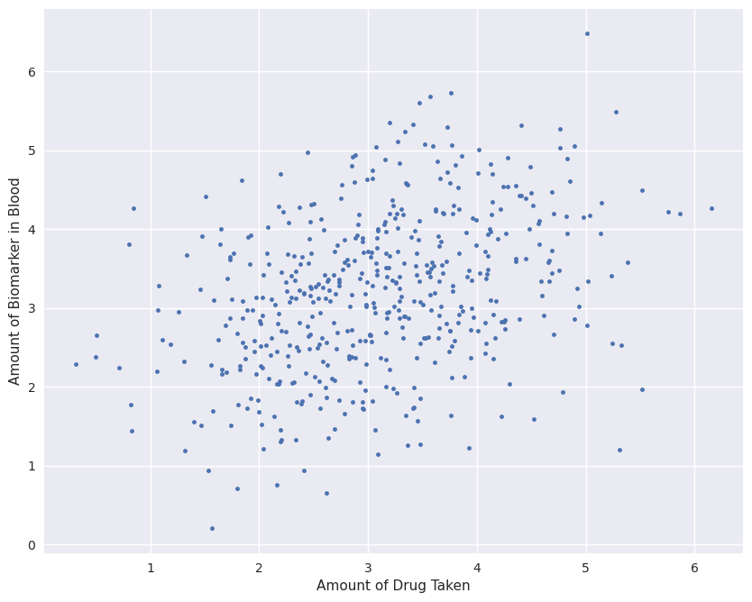
The first thing that we do to analyze the data is to find a linear best-fit. By performing a least-squares regression, the slope of the line will tell us whether the amount of drug taken is positively correlated with the amount of biomarker. We fit $Y=\beta X+\epsilon$ to this data, giving $\beta =0.375$:

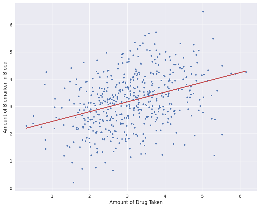
The slope is clearly positive, meaning that the people who took more of the drug fared better on average than those who didn’t. With this clear result, we happily give the new “miracle drug” to the entire population, which gives us a new dataset:

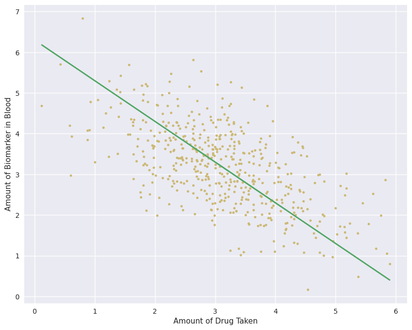
This new dataset (yellow points) seems to show the opposite result from the original data (blue points). There is a clear negative correlation between the amount of drug taken and the biomarker of interest, meaning that the drug actually hurts people! What went wrong with the original dataset? Or, more importantly, given only the original data (blue points), could we have found out that this drug is harmful? The question of whether we can find the true causal effect from only observational data is usually called the problem of “identification”.

This problem is impossible to solve without information beyond the data, namely our knowledge of the context in which the original data was gathered. Here we will encode this knowledge through what are known as “Structural Causal Models”.

Encoding Context: Structural Causal Models

Here, we focus on linear models. A linear Structural Causal Model (SCM), is a system of linear equations that encodes assumptions about the causal relationships between variables. When performing the linear regression, we implicitly assumed that the amount of drug taken, $X$, and the amount of biomarker in blood, $Y$, are causally related as follows:

$$\begin{array}{rl}X& :={ϵ}_x\\ Y& :={\lambda }_{xy}X+{ϵ}_y\end{array}$$ $${ϵ}_x,{ϵ}_y\text{uncorrelated}$$

In the above, ${\lambda }_{xy}$ represents the direct causal effect of $X$ on $Y$. Here it is the amount that $Y$ changes per unit change in $X$. The $ϵ$ in the equations summarizes the effects of unobserved causes. The assignment operator ($:=$) was used here because the equations are causal, and their effect only goes one way. That means that if we were to change the value of $Y$ directly (perhaps by injecting the person with the desired antibodies), it would not affect the value of $X$ (the amount of medicine the person took), but changing the amount of medicine they take does change their antibody count. Critically, we assumed that ${ϵ}_x$ is independent of ${ϵ}_y$, meaning that there are no unobserved common causes of both variables.

Let’s see what a linear regression computes here. We set up the regression equation: $Y=\beta X+\epsilon$, with the hope that the solved value is $\beta ={\lambda }_{xy}$. A least-squares regression finds the value of $\beta$ that minimizes $(Y-\beta X{)}^2$ over the entire dataset. In other words,

$$\beta =\underset{\beta }{\mathrm{argmin}}\frac{1}{n}\sum _{i=1}^n(y_i-\beta x_i{)}^2=\underset{\beta }{\mathrm{argmin}}\mathbb{E}[(Y-\beta X{)}^2]$$

Recall that the covariance between $X$ and $Y$ is defined ${\sigma }_{xy}=\mathbb{E}[(X-\mathbb{E}[X])(Y-\mathbb{E}[Y])]=\mathbb{E}[XY]-\mathbb{E}[X]\mathbb{E}[Y]$. To simplify the math (without loss of generality), let’s assume that $X$ and $Y$ are normalized, meaning that the data has mean 0 and variance 1. This makes ${\sigma }_{xy}=\mathbb{E}[XY]$. With this, we can derive the solution to $\beta$ with a bit of calculus, which gives:

$$\beta ={\sigma }_{xy}$$

Show the derivation

Start out by expanding out the least-squares equation, exploiting the fact that normalized variables have variance 1:

Then, to find the value of $\beta$ that minimizes this, take the derivative:

A regression computes the covariance between variables when variables are normalized… What does that have to do with ${\lambda }_{xy}$? It turns out that the covariances and structural coefficients (${\lambda }_{xy}$) in the equations underlying the data are deeply related:

$${\sigma }_{xy}=\mathbb{E}[XY]=\mathbb{E}[X({\lambda }_{xy}X+{ϵ}_y)]={\lambda }_{xy}\mathbb{E}[XX]+\mathbb{E}[{ϵ}_x{ϵ}_y]={\lambda }_{xy}$$

Here, the covariance of $X$ and $Y$ matches the causal effect of $X$ on $Y$. This seems to imply that the analysis done in section 1 was correct, so why did it give the wrong answer?

It turns out that the medicine in question is extremely expensive, so only the rich can afford to take large amounts. Wealthy people are more likely to get better anyways, simply because they don’t need to keep working while they’re sick, and can focus on recovery! The true model was in fact:

$$\begin{array}{rl}X& :={ϵ}_x\\ Y& :={\lambda }_{xy}X+{ϵ}_y\end{array}$$ $${ϵ}_x,{ϵ}_y\text{correlated}$$

Since wealth was not gathered as part of the dataset, it is a latent confounder, represented by a correlation between the $ϵ$ values, and is shown in the causal graph as a bidirected dashed edge. Now, defining ${ϵ}_{xy}\equiv \mathbb{E}[{ϵ}_x{ϵ}_y]$, the regression gives us:

$$\beta ={\sigma }_{xy}={\lambda }_{xy}\mathbb{E}[XX]+\mathbb{E}[{ϵ}_x{ϵ}_y]={\lambda }_{xy}+{ϵ}_{xy}$$

The first term in the result, ${\lambda }_{xy}$, is the causal effect of the drug, which we are after; but the second, ${ϵ}_{xy}$, is the effect of wealth on both taking the drug, and getting the biomarker, which is not what we wanted. Unfortunately, without any more information, it is impossible to disambiguate between the two (one equation, two unknown variables), meaning that we can’t tell how much of the correlation comes from the casual effect of the drug, and how much from the confounding. In this situation, we call ${\lambda }_{xy}$ not identifiable. In other words, there is no way to find what would happen if the drug were given to everyone, independently of their wealth.

One fix for this would be to gather the wealth data explicitly from every person in the study. However, some people might not want to share such information. All is not lost, though. Suppose each subject in the study has a doctor who recommended taking the drug lightly, strongly, or anywhere in between. The amount of the drug they took was directly influenced by their doctors’ recommendation. Critically, the decision of the doctor was not based on the wealth of the patients, or other confounders (e.g, the doctor was recommending the drug for another condition, unrelated to the biomarker of interest). If we gather a new dataset which includes this recommendation level, we get:

$$\begin{array}{rl}Z& :={ϵ}_z\\ X& :={\lambda }_{zx}Z+{ϵ}_x\\ Y& :={\lambda }_{xy}X+{ϵ}_y\end{array}$$ $${ϵ}_x,{ϵ}_y\text{correlated}$$ $${ϵ}_z,{ϵ}_x\text{ and }{ϵ}_z,{ϵ}_y\text{uncorrelated}$$

In this situation, regressing $Y$ on $X$ is still biased. Nevertheless, we can combine the data in a different way to obtain the causal effect:

$${\sigma }_{zy}=\mathbb{E}[ZY]=\mathbb{E}[Z({\lambda }_{xy}X+{ϵ}_y)]={\lambda }_{xy}\mathbb{E}[ZX]+\mathbb{E}[{ϵ}_z{ϵ}_y]$$$${\sigma }_{zy}={\lambda }_{xy}{\sigma }_{zx}\Rightarrow {\lambda }_{xy}=\frac{{\sigma }_{zy}}{{\sigma }_{zx}}$$

If our model is right, the desired causal effect can be solved as a ratio of two covariances/regressions! This method is usually called the instrumental variable, and is extremely common in the literature [1]. Estimation of that ratio is typically achieved using 2-stage least squares.

2-Stage Least Squares

As the name suggests, rather than using a ratio of two regressions, a 2SLS uses the result of one regression to adjust the other. In particular, first the regression $X={\beta }_{x}Z+\epsilon$ is performed, which gives ${\beta }_x={\sigma }_{xz}$.

Then, the resulting ${\beta }_{x}Z$ is plugged into another regression equation, replacing $X$:

$$Y={\beta }_y({\beta }_{x}Z)+\epsilon \Rightarrow Y={\beta }_y({\sigma }_{xz}Z)+\epsilon$$

If we were to perform a regression $Y=\beta Z+\epsilon$, we would get $\beta ={\sigma }_{zy}$. We know from the definition of least-squares that this value minimizes $\mathbb{E}[(Y-\beta Z{)}^2]$. So what value would minimize the compounded regression?

$$\underset{\beta }{\mathrm{argmin}}\mathbb{E}[(Y-{\beta }_y({\sigma }_{xz}Z){)}^2]=\underset{\beta }{\mathrm{argmin}}\mathbb{E}[(Y-({\beta }_y{\sigma }_{xz})Z{)}^2]$$$${\sigma }_{zy}={\beta }_y{\sigma }_{zx}\Rightarrow {\beta }_y=\frac{{\sigma }_{zy}}{{\sigma }_{zx}}$$

Despite the procedure being different, the end effect is the same: the resulting value corresponds to the same ratio of covariances that was derived above.

In general, no single regression gives the desired answer, it is only through a clever combination of steps based on the underlying causal model that an adjustment formula can be derived, giving the causal effect.

Finding this adjustment formula, given our model of the world (structural equations and causal graph) is the goal of identification. If such a formula exists, an identification algorithm would return it, and if not, the algorithm would say that the desired effect cannot be found.

Most state-of-the-art methods for identification look for patterns in the causal graph which signal that mathematical tricks like the one shown above can be used to solve for a desired parameter. Such graphical methods focus on paths and flows between sets of variables, as will be demonstrated in the next section.

Auxiliary Variables

Suppose we have the following structural model, and want to find the causal effect of $X$ on $Y$, ${\lambda }_{xy}$.

$$\begin{array}{rl}Z& :={ϵ}_z\\ X& :={\lambda }_{zx}Z+{ϵ}_x\\ Y& :={\lambda }_{xy}X+{ϵ}_y\end{array}$$ $${ϵ}_z,{ϵ}_y\text{correlated}$$ $${ϵ}_z,{ϵ}_x\text{ and }{ϵ}_x,{ϵ}_y\text{uncorrelated}$$

Expanding out the covariance between $X$ and $Y$ gives ${\sigma }_{xy}={\lambda }_{xy}+{\lambda }_{zx}{ϵ}_{zy}$. This is a combination of the causal effect ${\lambda }_{xy}$, and the back-door path from $X$, to $Z$, to $Y$, namely ${\lambda }_{zx}{ϵ}_{zy}$ (this can be read directly off of the causal graph, see path analysis [2]).

Experts in the field might notice that a simple regression of $Y$ on $X$ adjusting for $Z$ gives ${\lambda }_{xy}$ (known as the backdoor adjustment [3]). We will approach the problem from a different angle, which turns out to be easily extensible to complex models where conditioning fails. Our goal is to somehow remove the effect of ${\lambda }_{zx}{ϵ}_{zy}$ from ${\sigma }_{xy}$, which will leave only the desired parameter.

We turn to Auxiliary Variables [4], allowing usage of previously-solved parameters to help solve for others. In this example, ${\sigma }_{zx}={\lambda }_{zx}$, so we have solved the causal effect of $Z$ on $X$. We use this to define a new “Auxiliary” variable $X^{\ast }=X-{\lambda }_{zx}Z$, which subtracts the effect of $Z$ on $X$, and has a cool property:

$$X^{\ast }=X-{\lambda }_{zx}Z=({\lambda }_{zx}Z+{ϵ}_x)-{\lambda }_{zx}Z={ϵ}_x$$

This new variable $X^{\ast }$ behaves as if it were not affected by $Z$ at all - as if the edge ${\lambda }_{zx}$ were missing in the causal graph. This means that the covariance of $X^{\ast }$ and $Y$ no longer includes the backdoor path, and can be used to compute the desired value similarly to an instrumental variable:

$$\frac{{\sigma }_{x^{\ast }y}}{{\sigma }_{x^{\ast }x}}=\frac{\mathbb{E}[X^{\ast }Y]}{\mathbb{E}[X^{\ast }X]}=\frac{\mathbb{E}[X^{\ast }({\lambda }_{xy}X+{ϵ}_y)]}{\mathbb{E}[X^{\ast }X]}=\frac{{\lambda }_{xy}\mathbb{E}[X^{\ast }X]}{\mathbb{E}[X^{\ast }X]}={\lambda }_{xy}$$

This method misses some simple cases, though.

Total Effect AV

And here, finally, is where our paper’s contributions begin. In the following example, the edges incoming into $X$ in the causal graph, ${\lambda }_{wx}$ and ${\lambda }_{zx}$, cannot be solved, meaning that no AV $X^{\ast }$ can be created:

$$\begin{array}{rl}W& :={ϵ}_w\\ Z& :={\lambda }_{wz}W+{ϵ}_z\\ X& :={\lambda }_{wx}W+{\lambda }_{zx}Z+{ϵ}_x\\ Y& :={\lambda }_{xy}X+{ϵ}_y\end{array}$$ $${ϵ}_z,{ϵ}_x\text{correlated}$$ $${ϵ}_w,{ϵ}_y\text{correlated}$$

Nevertheless, the total effect of $W$ on $X$, denoted by ${\delta }_{wx}={\lambda }_{wx}+{\lambda }_{wz}{\lambda }_{zx}$ is simply ${\sigma }_{wx}$, so we can create a new type of AV,

$$X^{†}=X-{\delta }_{wx}W$$

Once again, a bit of math shows that this AV can be used to successfully solve for the desired ${\lambda }_{xy}$:

Of course, the situation becomes much more complex once there are multiple back-door paths between $X$ and $Y$. The following graph has back-door paths between $X$ and $Y$ passing through $A$ and $D$, but if we try defining a total-effect AV by individually subtracting out total effects, $X^{‡}=X-{\delta }_{ax}A-{\delta }_{dx}D$, we get a biased answer:

The path in purple is double-subtracted!

The key insight needed to solve this problem is that the total-effect of $A$ on $X$ has a part passing through $D$ - but that part of the effect is already removed when subtracting ${\delta }_{dx}D$! This means that the correct approach is subtracting out a partial effect - the portion of the effect of $A$ on $X$ that does not pass through $D$, denoted by ${\delta }_{ax.d}$, which gives the AV $X^{†}=X-{\delta }_{ax.d}A-{\delta }_{dx.a}D$

Yay, it worked!

This is all great, but how exactly does one find the value of these partial effects, so that they can be removed from $X$?

Partial Effect Instrumental Set (PEIS)

The PEIS is a method to find exactly the partial effects needed to contruct the proposed new AVs. We assume that readers of this section are familiar with instrumental sets [5], or have read the “Unconditioned Instrumental Sets” section of the post from our previous paper. The core takeaway of that section is repeated here:

In an instrumental set, a system of linear equations is created for parents of target $Y$, which can be used to solve for incident edges ${\lambda }_{x_{1}y}$ and ${\lambda }_{x_{2}y}$:

It turns out that the exact same type of system will solve for the desired partial effects! The main difference now is that instead of being restricted to parents of the target (as in the IS), we can use any nodes. In this case, we use $A$ and $D$, since those are the non-intersecting partial effects we want to find. Next, we recognize that $A$ and $B$ have all of their paths to $X$ pass through $A$ and $D$ (can’t use $D$ instead of $B$, since it has bidirected edge to $X$). We proved that this means we can construct the following system of equations, which gives precisely the desired result:

$$\begin{array}{rl}{\sigma }_{ax}& ={\sigma }_{aa}{\delta }_{ax.d}+{\sigma }_{ad}{\delta }_{dx.a}\\ {\sigma }_{bx}& ={\sigma }_{ba}{\delta }_{ax.d}+{\sigma }_{bd}{\delta }_{dx.a}\end{array}$$

With the PEIS and the total-effect AVs as defined above, it is now possible to identify a new class of parameters missed by previous efficient approaches.

Auxiliary Cutsets & ACID

Our paper uses these insights to develop a new algorithm for identification which recursively finds total-effect AVs, identifying successively more parameters in each iteration. Surprisingly, this method turns out to subsume the generalized conditional instrumental set, which has unknown computational complexity, and has NP-Hard variants [6 kumorEfficientIdentificationLinear2019]. Critically, our algorithm finds optimal total-effect AVs and their corresponding PEIS in polynomial-time, being the first efficient method that subsumes generalized instrumental sets.

In fact, to the best of our knowledge, it subsumes all polynomial-time algorithms for identification in linear SCM, as can be seen in this figure taken from the paper:

To find out details of our algorithm, and to see how all of this was proved, please refer to the paper!

---

References

1. Angrist, J. D., Imbens, G. W., & Rubin, D. B. (1996). Identification of Causal Effects Using Instrumental Variables. Journal of the American Statistical Association, 91(434), 444–455. https://doi.org/10.2307/2291629
2. Wright, S. (1921). Correlation and Causation. Journal of Agricultural Research, 20(7), 557–585.
3. Pearl, J. (2000). Causality: Models, Reasoning and Inference.
4. Chen, B., Pearl, J., & Bareinboim, E. (2016). Incorporating Knowledge into Structural Equation Models Using Auxiliary Variables. IJCAI 2016, Proceedings of the 25th International Joint Conference on Artificial Intelligence, 7.
5. Brito, C., & Pearl, J. (2002). Generalized Instrumental Variables. Proceedings of the Eighteenth Conference on Uncertainty in Artificial Intelligence, 85–93.
6. Van der Zander, B., & Liśkiewicz, M. (2016). On Searching for Generalized Instrumental Variables. Proceedings of the 19th International Conference on Artificial Intelligence and Statistics (AISTATS-16).